
I recently studied mortality and population curves in T. Waldron’s “Counting the Dead” (1994) [for reasons not related to this post]. That got me thinking about how pandemics impact the demographic profile osteologists derive from cemeteries, mass graves, and past populations.
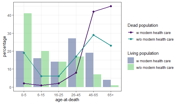
But first we must consider what we would expect to see in a ‘normal’ population. In societies without access to modern healthcare we generally expect a U shaped pattern (many die young and many die “old”) whereas access to modern healthcare skews the curve to predominantly older people dying.
Among the living, the demographics of those without access to modern healthcare is almost an inverted mirror image, with many children, juveniles, and young adults (sometimes up to 45/50%) and few individuals over 45. Whereas living populations who have modern healthcare maintain larger populations in age groups above 25 years old.
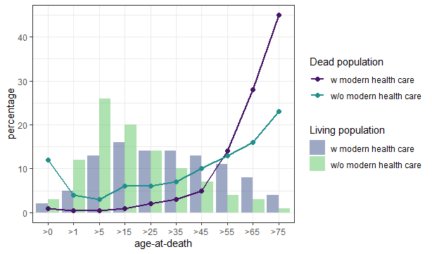
(based on Waldron 1994:17-19)
Observe the difference of not only the different age structures of a living and it’s dead population. Additionally, keep in mind that this data is not continous, the living population is a “one shot picture”, and the dead population has accumulated over time. Details at the end of the post.
Based on the few early historic sources on infant and child mortality, it is estimated that between 30 – 60 % of all individuals born did not reach the age of 25. Nonetheless a percentage this high is rarely seen in bioarchaeology, mainly due to factors affecting survival and visibility of remains (taphonomy) the bones are very fragile and many societies treat dead children different from adults (e.g. the Christian eaves burial or Romans burying infants in their homes). Individuals surviving childhood have different life expectancies, depending on the time and place they happen to be alive. Often, the overall young mean age-at-death of archaeological populations is strongly influenced by high infant/child mortality and there were people over 60 or even 80. Further a normal demographic profile should be close to 1:1 of male: female sex estimations, strong deviations from that indicate gender specific burial practices (e.g. burial grounds of religious orders often show a strong preference of one sex). However, one should be careful if the sample size is small.
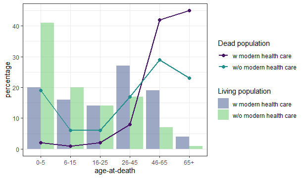
Whilst these percentages are quite informative, observable bioarchaeological age estimation does not pan out in quite the same way. Though teeth allow close estimates, without forensic methods ie based soley on morphology it is very hard to estimate an adults age with any accuracy. Meaning, resultant demographic models will look less smooth and a lot more boxy. Whatsmore, if we attempt to plot pathologies, one of the most important things in identifying broader pandemic trends, it should be noted that mortality rates (in epidemiology) are always given as death rate per 100 000 individuals, not in percentages. Further, most diseases with aggressive mortality are not traceable via skeletal remains. Bone needs around 10-14 days to react to infections and diseases, so for most skeletons the cause of death cannot be defined. People with archaeologically visible signs of e.g. infected sinuses are actually “survivors” and not people who immediatley succumed to illness. We call it the “osteological paradox” as it creates problems in attributing graves to historically known pademics.
However, despite the aforementioned caveats and complexities of the osteological examination of populations, there are graves with associated historic evidence, such as the Black Death mass grave from East Smithfield in London which provide some insight. Here, examination revealed a demography which followed that of a normal population and associated risk of death increased with age.
We can compare this Medieval archaeological data to a more recent pandemic with more detailed demographic data on ‘age at death’ by examining the mortality rates of the Spanish Flu. Whilst having a different global dissemination, distribution and being the result of a different disease, it results in a demographic picture similar to the Black Death. Note in the fact, that the same age groups were affected (life expectancy had drastically increased by the early C20th) but the observable death rate per age group is an amplified version of the previously existing death rates, meaning it affected all age groups equally. However, it should be noted that working with profiles from the Spanish Flu is difficult as at the same time WWI devastatingly altered the demography of Europe.
I choose these examples specifically, because they are among the few that are recognisable, not only through historic references but also their mass graves. This burial type is perhaps one of the most significant tools of tracing unknown pandemics in (pre-)history, if the culture it originates from generally prefers single burials over multiple burials, there are no other obvious causal explanations, such as weapons trauma etc., (and sometimes: odd burial location) as it implicates a greater number of dead people in short time who could not be buried “the normal way”. What remains hidden are smaller events that allow the society to bury their dead as usual and pandemics that affect smaller groups within a society. In bioarchaeology both would lead to a higher death rate overall and maybe a deviation from the 1:1 sex estimate, if the disease is more likely to transmit to people of the same sex or one sex has a greater chance of survival.
– Chiara
The graphs…
Here is a bit more detail on the creation of the graphs and their literature. Both were developed on the data supplied in T. Waldron (1994) Counting the Dead: The Epidemiology of Skeletal Populations (Wiley) pages 17 (living populations of Peru and England&Wales, male data) and 19 (associated dead populations) by eyeballing the percentages. He choose them as examples for a “non developed” and a “developed” society, stating that the former should reflect the archaeological record and as time progresses the profile will change. As this is associated with general lifestyle and subsistence but mostly the access to healthcare I decided to avoid that wording and go with healthcare instead.
The data was collected in an excel sheet, imported in R, processed, and visualised with ggplot2 with viridis colours.


Leave a Reply